Retrieving the Green's function

Roel Snieder*
Center for Wave Phenomena and Department of Geophysics, Colorado School of Mines, Golden, Colorado 80401, USA
(Received 5 July 2006; revised manuscript received 9 August 2006; published 27 October 2006)

It is known that the Green's function for nondissipative acoustic or elastic wave propagation can be extracted
by correlating noise recorded at different receivers. This property is often related to the invariance for time
reversal of the acoustic or elastic wave equations. The diffusion equation is not invariant for time reversal. It
is shown in this work that the Green's function of the diffusion equation can also be retrieved by correlating
solutions of the diffusion equation that are excited randomly and are recorded at different locations. This
property can be used to retrieve the Green's function for diffusive systems from ambient fluctuations. Potential
applications include the fluid pressure in porous media, electromagnetic fields in conducting media, the diffusive
transport of contaminants, and the intensity of multiply scattered waves.

I. INTRODUCTION
The Green's function for acoustic or elastic waves can be
extracted by cross correlating recorded waves that are excited
by a random excitation; see Ref. [1], for a tutorial.
Derivations of this principle have been presented based on
normal modes [2], on representation theorems [3-5], on
time-reversal invariance [6,7], and on the principle of stationary
phase [8-10]. This technique has found applications
in ultrasound [11-13], crustal seismology [14-18], exploration
seismology [19,20], structural engineering [21,22], and
numerical modeling [23]. Recently, the extraction of the
Green's function by cross correlation has been derived for
general coupled systems of linear equations [24].

The principle of extracting the Green's function of a system
from ambient fluctuations creates the possibility to retrieve
the impulse response of a system without using controlled
point sources. This impulse response can be used for
imaging, tomography, or other methods to determine the
properties of the medium. For example, models of the crust
in California have been constructed using surface wave tomography
based on microseismic noise [15,18]. The autocorrelation
of ambient seismic noise has been used for daily
monitoring of fault zones [25] and volcanoes [26]. The
Green's function extracted from ambient noise can also be
used to model the response of a system to a prescribed excitation
without knowing the in situ properties of the system.

The extraction of the Green's function from ambient noise
has been described extensively for wave propagation of
acoustic or elastic waves without intrinsic attenuation (e.g.,
[1-10]). In the absence of intrinsic attenuation, the wave
equation is invariant for time reversal, and several derivations
of the reconstruction of the Green's function are indeed
based on time-reversal invariance [6,7,20].

Many physical systems are not invariant under time reversal.
Intrinsic attenuation breaks the symmetry for time reversal
for acoustic and elastic wave propagation. Electrical conductivity
breaks the time-reversal symmetry of Maxwell's
equations. It has been shown theoretically [27] and observationally
observa-tionally [21,22] that the impulse response of attenuating
waves can be retrieved from ambient fluctuations.
Time-reversal invariance is, however, not essential for retrieving
the Green's function from ambient noise. This can
be seen by considering the diffusion equation

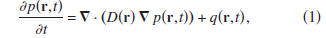
where the diffusion constant D may depend on position r.
The diffusion equation is not invariant for time reversal because
the operation t→ -t changes the sign of the first term.
Equation (1) is of practical importance because it describes
conductive heat transport, diffusive transport of tracers and
contaminants, fluid flow in porous media [28], electromagnetic
waves in conducting media [29], and the energy transport
of multiply scattered waves, e.g., [30].

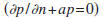
The derivation in this work is applicable to the frequency
domain, and the following Fourier convention is used:
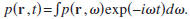With this convention, the diffusion
equation is, in the frequency domain, given by

Time reversal corresponds, in the frequency domain, to complex
conjugation. The time-reversed diffusion equation is
thus given by

where the asterisk denotes complex conjugation. The sign
difference in the first terms of expressions (2) and (3) is due
to the lack of time-reversal invariance of the diffusion equation.
It is shown here that the Green's function for the diffusion
equation can be retrieved by correlating noise recorded at
several locations in a diffusive system. One application of
this technique is monitoring flow in porous media. We therefore
refer to the solution of the diffusion equation as pressure,
but the results are equally valid for other diffusive systems.
In the following, all expressions are given in the
frequency domain, and the frequency dependence is not
shown explicitly.

II. REPRESENTATION THEOREMS
OF THE CONVOLUTION AND
CORRELATION TYPE
Following Fokkema and van den Berg [31,32], we consider
representation theorems of the convolution and correlation
types by using expressions (2) and (3) for two solutions
p_A and p_B with source terms q_A and q_B, respectively.
The representation theorem of the convolution type is obtained
by computing 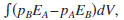where E_A denotes
Eq. (2) for state A, and where denotes an integration
over volume V. This gives

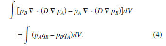
Note that in the subtraction the terms cancel. Applying
an integration by parts to the left-hand side of expression (4)
and using Gauss's theorem gives

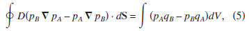
where the integral is over the surface that bounds
volume V.
A representation theorem of the correlation type can be
obtained by evaluating 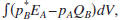where Q_B denotes
Eq. (3) for state B. Carrying out an integration by parts gives

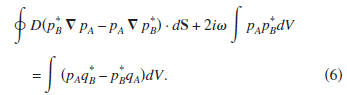
Note that now the iω terms in expressions (2) and (3) do not
cancel, but combine to give the volume integral in the lefthand
side. The presence of this term results from the lack of
invariance of time-reversal of the diffusion equation.
In the following integration over all space is used. The
contribution of the surface integral vanishes because the solution
of the diffusion equation p(r,ω) vanishes exponentially
as r→∞. Therefore, the representation theorems (5)
and (6) reduce to

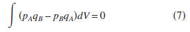
and

The contribution of the surface integral also vanishes for a
finite volume in case the solution satisfies either Dirichlet
conditions (p=0), Neumann conditions or mixed
boundary conditions at the surface that
bounds the volume.

III. REPRESENTATION THEOREMS
AND GREEN'S FUNCTIONS
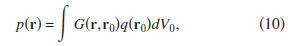
The Green's function for the diffusion equation is the solution
to Eq. (2) when the forcing is a function,

Setting 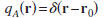in expression (7) implies that p_A(r)
=G(r,r₀). For this choice of q_A, expression (7) reduces to

where the subscripts B are dropped. Alternatively, setting

implies that

For this choice of the states A and B, expression (7) reduces
to the reciprocity relation,

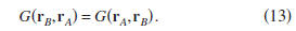
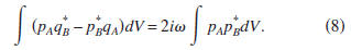
Inserting the states (12) into expression (8) gives

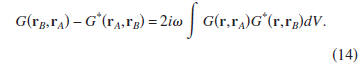
Using reciprocity, this expression can also be written as

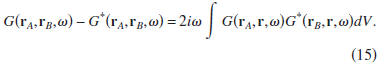
The left-hand side of Eq. (15) corresponds, in the time domain,
to the superposition of the Green's function and the
time-reversed Green's function. In Sec. IV, we consider how
this superposition can be retrieved from the cross correlation
of the pressure generated by uncorrelated sources.

IV. RETRIEVING THE GREEN'S FUNCTION
In order to show how the Green's function can be extracted
from the correlation of solutions generated by random
sources, let us consider spatially uncorrelated sources
with power spectrum that does not depend on location,

where the angular brackets denote the expectation value. In
practical applications, this expectation value is usually replaced
by using several nonoverlapping time windows (e.g.,
[33,26]). Multiplying Eq. (15) with , the volume integral
in that expression can be written as

RETRIEVING THE GREEN'S FUNCTION OF THE&[8230;

When we use this result and expression (10), Eq. (15) after
multiplication with is given by

where p(r,ω) is the pressure at location r due to the random
forcing q(r,ω).

Equation (18) states that the superposition of the Green's
function G(r_A,r_B,ω) and its time-reversed version is, after
multiplication with the power spectrum of the excitation,
equal to the correlation of the random fields at locations r_A
and r_B, respectively. The prefactor 2iω corresponds, in the
time domain, with -2d/dt. Since multiplication in the frequency
domain corresponds, in the time domain, to convolution
expression (19), in the time domain, is given by

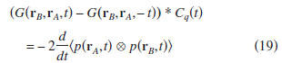
where the asterisk denotes convolution, denotes correlation,
and C_q(t) is the autocorrelation of _q(t).

V. DISCUSSION
The Green's function of the diffusion equation can be
retrieved by cross correlating measurements of a diffusive
system that is excited by random noise. Since the diffusion
equation is not invariant for time reversal, this shows that
invariance for time reversal is not essential for the retrieval
of the Green's function by cross correlation.

For elastic and acoustic waves, the Green's function can
be extracted from waves that are excited randomly at the
surface that surrounds the volume [3,5]. This is not the case
for the diffusion equation. For a volume of radius R, the
surface area grows with R^2, but for a homogeneous medium
the solution of the diffusion equation varies with the radius
as 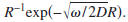The contribution of the surface integral
therefore depends on the radius of the volume, and the
derivation shown here holds for an infinite volume (R→∞),
or for a finite volume when Dirichlet, Neumann, or mixed
boundary conditions hold at the surface that bounds the vol-ume.
In contrast to the retrieval of the Green's function for
nonattenuating acoustic or elastic waves, where one needs
random sources on a surface that bounds the volume, one
needs random sources throughout the volume for the retrieval
of the Green's function for the diffusion equation.

The theory presented here provides an example that time-reversal
invariance is not required for the extraction of the
Green's function from ambient fluctuations. The diffusion
equation governs physical systems of practical importance,
and the derivation presented here makes it possible to retrieve
the impulse response of diffusive systems from measured
fluctuations.

In this work, the phrase pressure is used for the solution
of the diffusion equation because the pore pressure in a porous
medium follows the diffusion equation. The theory of
this work makes it possible to retrieve the Green's function
for fluid flow in an aquifer or hydrocarbon reservoir from
recorded pressure fluctuations. This Green's function can be
used to estimate parameters such as hydraulic conductivity
and to model the fluid transport in the subsurface without
explicit knowledge of the in situ hydraulic conductivity.
Similarly, the impulse response for the diffusive transport of
contaminants can be retrieved from observations of ambient
fluctuations in the concentration. The Green's function thus
obtained can then be used to predict the diffusive transport of
a localized release of the contaminant.

Electromagnetic fields in a conducting media satisfy the
diffusion equation. This has been used in the magnetotelluric
method where the ambient fluctuations in the electric and
magnetic fields observed at one location are used to determine
the electrical conductivity [34]. The theory presented
here makes it possible to retrieve the Green's function for
electromagnetic fields for noncoincident points from observed
electromagnetic fluctuations.

The intensity of multiply scattered waves satisfies, for late
times, the diffusion equation. Controlled intensity fluctuations
of multiply scattered waves have been used to create
images of the spatial distribution of the diffusion constant.
This has found application in medical imaging, e.g., [35].
Instead of using controlled, spatially localized, sources for
the intensity of scattered waves, one may use the theory of
this work to use random spatially distributed sources instead.

As always, the application of the theory to these, and
other, applications faces implementation issues. The assumption
that the sources of the ambient fluctuations have a homogeneous
spatial distribution may not be satisfied in practical
applications. For applications where this condition is
satisfied, the theory can be used to extract the impulse response
of diffusive systems without using a controlled, localized,
source.

ACKNOWLEDGMENTS
The author appreciates the comments of Ken Larner. This
research was supported by the Gamechanger Program of
Shell International Exploration and Production Inc.

ROEL SNIEDER

[1] A. Curtis, P. Gerstoft, H. Sato, R. Snieder, and K. Wapenaar,
The Leading Edge 25, 1082 (2006).
[2] O. I. Lobkis and R. L. Weaver, J. Acoust. Soc. Am. 110, 3011
(2001).
[3] K. Wapenaar, Phys. Rev. Lett. 93, 254301 (2004).
[4] R. L. Weaver and O. I. Lobkis, J. Acoust. Soc. Am. 116, 2731
(2004).
[5] K. Wapenaar, J. Fokkema, and R. Snieder, J. Acoust. Soc. Am.
118, 2783 (2005).
[6] A. Derode, E. Larose, M. Campillo, and M. Fink, Appl. Phys.
Lett. 83, 3054 (2003).
[7] A. Derode, E. Larose, M. Tanter, J. de Rosny, A. Tourin, M.
Campillo, and M. Fink, J. Acoust. Soc. Am. 113, 2973 (2003).
[8] R. Snieder, Phys. Rev. E 69, 046610 (2004).
[9] P. Roux, K. G. Sabra, W. A. Kuperman, and A. Roux, J.
Acoust. Soc. Am. 117, 79 (2005).
[10] R. Snieder, K. Wapenaar, and K. Larner, Geophysics 71,
SI111 (2006).
[11] R. L. Weaver and O. I. Lobkis, Phys. Rev. Lett. 87, 134301
(2001).
[12] A. Malcolm, J. Scales, and B. A. van Tiggelen, Phys. Rev. E
70, 015601(R) (2004).
[13] E. Larose, G. Montaldo, A. Derode, and M. Campillo, Appl.
Phys. Lett. 88, 104103 (2006).
[14] M. Campillo and A. Paul, Science 299, 547 (2003).
[15] N. M. Shapiro, M. Campillo, L. Stehly, and M. H. Ritzwoller,
Science 307, 1615 (2005).
[16] P. Roux, K. G. Sabra, P. Gerstoft, and W. A. Kuperman, Geophys.
Res. Lett. 32, L19303 (2005).
[17] K. G. Sabra, P. Gerstoft, P. Roux, W. A. Kuperman, and M. C.
Fehler, Geophys. Res. Lett. 32, L03310 (2005).
[18] K. G. Sabra, P. Gerstoft, P. Roux, W. A. Kuperman, and M. C.
Fehler, Geophys. Res. Lett. 32, L14311 (2005).
[19] A. Bakulin and R. Calvert, Geophysics 71, SI139 (2006).
[20] A. Bakulin and R. Calvert, Expanded Abstracts of 2004 SEGMeeting
(Society of Exploration Geophysicists, Tulsa, OK,
2004), pp. 2477-2480.
[21] R. Snieder and E. Safak, Bull. Seismol. Soc. Am. 96, 586
(2006).
[22] R. Snieder, J. Sheiman, and R. Calvert, Phys. Rev. E 73,
066620 (2006).
[23] D. J. van Manen, J. O. A. Robertsson, and A. Curtis, Phys.
Rev. Lett. 94, 164301 (2005).
[24] K. Wapenaar, E. Slob, and R. Snieder, Phys. Rev. Lett. (to be
published).
[25] U. Wegler and C. Sens-Schönfelder, Geophys. J. Int. (to be
published).
[26] C. Sens-Schönfelder and U. Wegler, Geophys. Res. Lett. (to be
published).
[27] R. Snieder, J. Acoust. Soc. Am. (to be published).
[28] H. F. Wang, Theory of Linear Poroelasticity, with Applications
to Geomechanics and Hydrogeology (Princeton University
Press, Princeton, 2000).
[29] J. D. Jackson, Classical Electrodynamics, 2nd ed. (Wiley, New
York, 1975).
[30] P. Sheng, Introduction to Wave Scattering, Localization, and
Mesoscopic Phenomena (Academic Press, New York, 1995).
[31] J. T. Fokkema and P. M. van den Berg, Seismic Applications of
Acoustic Reciprocity (Elsevier, Amsterdam, 1993).
[32] J. T. Fokkema and P. M. van den Berg, In Wavefields and
Reciprocity, edited by P. M. van den Berg, H. Blok, and J. T.
Fokkema (Delft University Press, Delft, 1996), pp. 99-108.
[33] N. M. Shapiro and M. Campillo, Geophys. Res. Lett. 31,
L07614 (2004).
[34] P. Weidelt, J. Geophys. Res. 38, 257 (1972).
[35] A. Yodh and B. Chance, Phys. Today 48(3), 34 (1995).
ROEL SNIEDER PHYSICAL REVIEW E 74, 046620 (2006)