Intersections of Tangent Lines of Exponential Functions

Tim Feeman received his Ph.D. in 1984 at the University of Michigan under Allen Shields and has been at Villanova University (Villanova, PA 19085) since 1986. His book Portraits of the Earth: A Mathematician Looks at Maps was published in 2002 by the American Mathematical Society. He is an avid runner and enjoys the cryptic crosswords in The Times (London).

Osvaldo Marrero studied mathematics at the University of Miami and biometry and statistics at Yale University. After holding positions in academia and in industry, he is currently a professor at Villanova University. He has published papers in epidemiology, mathematics, medicine, and statistics. Besides doing mathematical research, he enjoys listening to music, physical exercise, and travel. Fluent in English, French, and Spanish, he keeps trying to improve his knowledge of other languages.

Among the intriguing geometric properties of a parabola is this: if AB is any chord
of the parabola and L is the tangent to the parabola parallel to AB, then the midpoint of
the chord, the point of tangency of L, and the point where the tangents to the parabola
at A and at B intersect are collinear. Moreover, the line they form is parallel to the axis
of symmetry of the parabola. So, if we make the parabola’s axis of symmetry coincide
with the y-axis in a Cartesian coordinate system, then it follows that the x-coordinate
of these points is the average of the x-coordinates of A and B. (See Stein [2] for more
on this.)

In [3], Stenlund shows that, among all analytic curves, this property is unique to
parabolas. In discussing this result, Stenlund looks at a second curve associated with a
parabola. Specifically, fix a positive horizontal displacement h, and, for any chord AB
where the x-coordinates of A and B differ by h, look at the point where the tangents
to the parabola at A and at B intersect. The locus of all such intersections of pairs
of tangents forms another parabola, as Stenlund demonstrates. Moreover, this derived
parabola is a translation along the axis of symmetry of the original parabola by an
amount that depends on h. Figure 1 illustrates this construction for the parabola y = x²
with h = 2.

We wondered whether a parabola was the only curve for which this associated derived
curve was essentially a copy of itself, and thus we were led to consider exponential
functions.

Derived curves

We extend Stenlund’s construction to exponential functions. For k ≠ 0, let  .
Fix h > 0 and let t be an arbitrary real number. The lines tangent to the graph of g at

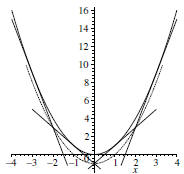
Figure 1. The parabola y = x² and its associated derived parabola y = x² − 1 corresponding
to the horizontal displacement h = 2.

the points (t − h/2, g (t − h/2)) and (t + h/2, g (t + h/2)) are

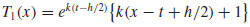
and

respectively. The x-coordinate of their intersection point is

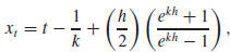
so its y-coordinate is

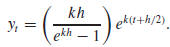
(The left-hand diagram in Figure 2 illustrates this construction.) We thus have parametric
equations for the associated derived curve, and we can easily eliminate t to get
y_t directly as a function of x_t . After simplifying, we have

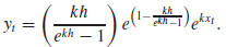
In summary, we have shown the following:

Theorem. Let h and k be real numbers with h > 0 and k ≠ 0, and let

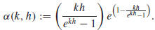
Then the derived curve for the exponential function

Thus, the derived curve of the exponential function g is also an exponential function,
and differs from g by the scaling factor α (k, h). Figure 2 gives an illustration.

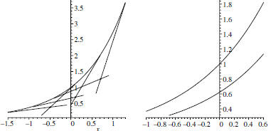
Figure 2. and its associated derived curve

The scaling factor α (k ,h)

We now consider the behavior of the scaling function α (k, h). To begin, let

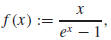for x≠0

Observe that f (x) > 0 for all nonzero x, and that  . Thus, we define
f (0) := 1 to get a function that is continuous on the real line.

That e^x − 1 > x for all nonzero x is a straightforward application of the Mean Value
Theorem. Therefore, 0 < f (x) ≤ 1 for x ≥ 0 and f (x) ≥ 1 for x ≤ 0. Moreover, an
application of l’’s Rule shows that  f'(0) = −1/2. Thus, f is differentiable
on R.

Now consider the function . Since , we see that p
attains its absolute maximum value at p(1) = 1. The substitution of f (x) for t shows
that the function   is differentiable and satisfies 0 < F (x) ≤ 1
on R. Also, F (x) = 1 only for x = 0.

Finally, let h, k, and α (k, h) be as in the theorem. Thus, α (k, h) = F (k h), whence
for each fixed value of k, as one would have hoped. In fact, the
equation α (k, h) = F (k h) extends α to a differentiable function in the k h-plane that
satisfies 0 < α (k, h) ≤ 1 and α (k, h) = 1 only when k h = 0. The level curves of the
graph of α are the hyperbolas k h = constant. The graph of α is shown in Figure 3.

In conclusion, we have shown that the derived curve associated with an exponential
function is again an exponential function, so this sort of invariance is not unique to
parabolas. Unlike the situation for parabolas, however, the derived curve of an expo-

Figure 3. The graph of α (k, h) for −4 ≤ k, h ≤ 4. Maple does not plot α(0, 0), which is
defined only as a limit. Note the hyperbolic level curves.

nential function is not a translation, but a rescaling of the original curve by a factor
whose properties we have analyzed.

In [4], Wilkins uses intrinsic geometric characterizations of the conic sections to
generalize the main results of [3]. He shows that the property of parabolas cited in
the opening paragraph of this article can be expressed as an angle-bisection property
that is unique to the conic sections. Lacking an intrinsic geometric formulation of the
derived curve of an exponential, we have been unable to determine whether or not the
exponentials are unique in possessing the property that the derived curve is a multiple
of the original curve.

References

1. T. L. Heath, The Works of Archimedes, Dover, 1953.
2. S. Stein, Archimedes: What Did He Do Besides Cry Eureka?, MAA, 1999.
3. M. Stenlund, On the tangent lines of a parabola, College Math. J. 32 (2001) 194–196.
4. D. Wilkins, The tangent lines of a conic section, College Math. J. 34 (2003) 296–303.