

Numerical Linear Algebra
3.5 – The Schur and Singular Value Decompositions
A related problem is computing the eigenvalues of a matrix. Computing the
eigenvalues of a matrix is more complicated than solving a set of linear
equations. We
can immediately see that no algorithm will be able to exactly compute the
eigenvalues of
a matrix. This is a direct consequence of Galois Theory, which proves that the
problem of
finding the roots of a polynomial of order 5 or larger does not admit a closed
form
expression in radicals. Now, recall that the eigenvalues of an n -dimensional
matrix can
be found by solving an n th order polynomial. Hence, we cannot expect an
algorithm of
the type we used for the LU and Cholesky decompositions. Actual algorithms for
computing the eigenvalues and singular value decomposition are iterative in
nature.
The actual algorithms for both cases are quiet complicated. Numerical recipes
actually suggests that this is one of the few areas where relying on black-box
code is
actually recommended.
It Table 3.5, we summarize the various linear algebra problems for a number of
different types of matrices.
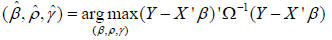
3.6 – Estimation of Linear ARMA Models
Consider the following time series regression model,
 where
where
 and
and  .
This process for
.
This process for is called a first-order moving average
process, or an MA1 process. Notice that,
Table 3.5 – Matrix Algorithms
| Factor | Solve Linear System | Compute Inverse | Compute Eigenvalues | Determinant | Condition Number | |
| General Matrix
|
LU O(n^3) dgetrf |
Tri. Solve O(n^2) given LU dgetrs |
Tri. Inverse O(n^3) given LU dgetri |
Schur Gen. Iterative dgeev |
Multiply Diag. O(n) given LU |
O(n^2) given LU dgecon |
| Sym. Indef.
|
BK O(n^3) dsytrf |
Spec O(n^2) given BK dsytrs |
Spec. O(n^3) given BK dsytri |
Schur. Symmetric Iterative dsyev |
???
|
O(n^2) given BK dsycon |
| Sym. Pos. Def.
|
Cholesky O(n^3) dpotrf |
Tri. Solve O(n^2) given Chold. dpotrs |
Cholesky O(n^3) given Chold dpotri |
Schur. Symmetric Iterative dsyev |
Multiply Diag. O(n) given Chold. |
O(n^2) given Chold. dpocon |
| Lower/Upper
|
N/A
|
Tri. Solve O(n^2) dtrsv (BLAS) |
Tri. Inverse O(n^3) dtrtri |
Direct O(n) |
Direct O(n) |
Direct O(n) dtrcon |
| Band
|
Band LU O(n*k^2) dgbtrf |
Tri. Band Solve O(n*k) given LU dgbtrs |
O(n^2*k) given LU dgbtri |
Schur Gen. Iterative dgeev |
Band LU O(n) given LU |
Band LU O(n*k) given LU dgbcon |
| Sym. Indef. Band
|
Band LU O(n*k^2) dgbtrf |
Tri. Band Solve O(n*k) given LU dgbtrs |
O(n^2*k) given LU dgbtri |
Schur Band Sym. Iterative dsbev |
Band LU O(n) given LU |
Band LU O(n*k) given LU dgbcon |
| Sym. Pos. Def. Band
|
Band Cholesky O(n*k^2) dpbtrf |
Band Cholesky O(n*k^2) dpbtrs |
Band Cholesky O(n^2*k) dpbtri |
Schur Band SPD Iter. dsbev |
Band Cholesky O(n^2*k) |
Band Cholesky O(n^2*k) dpbcon |
| Lower/Upper Band
|
N/A
|
Tri. Solve O(n*k) dtbsv (BLAS) |
???
|
Direct O(n) |
Direct O(n) |
Direct O(n) |
| Block Diagonal |
LU by Block O(b*nb^3) |
Tri. Solve by Block O(b*nb^2) |
Tri. Inv. By Block O(b*nb^3) |
??? |
Multiply Diag. O(n) |
LU by Block O(b*nb^2) |
| Toeplitz SPD |
Teop Chold O(n^2) |
|||||
| Band Toeplitz SPD |
Band Teop Chold. O(n*k) |
where,
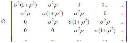
The maximum likelihood estimator is given by,
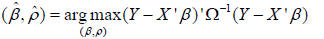
A naive approach to computing this estimator would form
Ω-1 using a standard
algorithm (e.g. the Cholesky decomposition). This system is special in a number
of ways.
First, the matrix Ω is band diagonal. A band diagonal matrix can be decomposed
in
O(nk2 ) operations instead of O(n3 ) where n is the number of rows and k is the
number
if bands. Second, forming Ω-1 using the band-Cholesky decomposition is not
efficient
either because the inverse of a band matrix is not necessarily a band matrix
with the same
number of bands. More generally, sparse matrices do not have sparse inverse.
Instead, we
can take the following approach. First, from the Cholesky decomposition Ω = LLT
using
the band Cholesky decomposition. This decomposition preserves the banded
structure.
Next, compute v = Y − X 'β . Third, solve Lx = v for x . This can be preformed
in O(nk)
operations. Finally, evaluate the likelihood function as x ' x . All the
operations together
mean that the likelihood can be evaluated in O(n) operations, since k is fixed
at 2.
Now consider the more general problem of the ARMA(1,1)
model. We have
 where
where  and
and
 . In
this case, we have,
. In
this case, we have,
where,
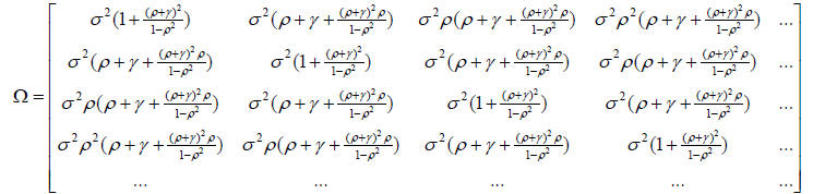
This matrix is no longer a band diagonal matrix. It is,
however, a Toeplitz matrix. Hence,
we can apply a similar procedure to the one above. In this case, we have an O(n2
)
algorithm for the Cholesky factorization. When T is quite large, then the
elements far
away from the diagonal will get quite small. Suppose that we trim all elements
that are
less than 0.0001 . In this case, we will have a band Toeplitz matrix. We can
then compute
the Cholesky decomposition in O(nk) operations. This is a huge difference from
the
naïve O(n3 ) ! For example, when n =1,000 and k = 30 , then

3.7 – Solving Linear Differential Equations
Initial Value Problems
A linear first order differential equation can be written as,
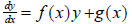
The simplest method of solving such an equation is to use finite difference
methods. We
compute a solution ![]() on
a grid of equally spaced points
on
a grid of equally spaced points  with a spacing of
 . We can then approximate
  using k
 .
Using this, we can write,
.
Using this, we can write,
This system will be pinned down if we specify  . Then, we can compute all
future
. Then, we can compute all
future
values using  . This type of problem is
called an initial value
. This type of problem is
called an initial value
problem, because it can be solved by iteration.
Boundary Value Problems
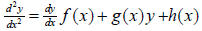
The above example is somewhat atypical. In most social science applications, we
have a second order derivative as follows,
We can similarly use a finite difference scheme to give,
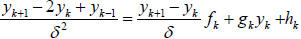
We can rearrange this to give,

If we have the values ![]() and
and
 , then we can solve the system by iteration.
Usually, this
, then we can solve the system by iteration.
Usually, this
is not the case, however. In most real problems, we have boundary value
problems.
Suppose that we have ![]() and
and
 . It turns outs that combining the above
equation with
. It turns outs that combining the above
equation with
the equation ![]() = a and
= b , we have a tri-diagonal system of linear
equations. This
= a and
= b , we have a tri-diagonal system of linear
equations. This
turns out to be a rather generally property of boundary value problems- they can
be
solved by applying band-diagonal factorizations.