MATRIX ALGEBRA:DETERMINANTS,INVERSES,EIGENVALUES

§C.4 EIGENVALUES AND EIGENVECTORS

Consider the special form of the linear system (C.13) in which the right-hand side vector y is a multiple
of the solution vector x:

Ax = λx, (C.48)

or, written in full,

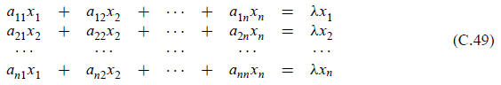
This is called the standard (or classical) algebraic eigenproblem. System (C.48) can be rearranged into
the homogeneous form

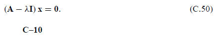
A nontrivial solution of this equation is possible if and only if the coefficient matrix A−λI is singular.
Such a condition can be expressed as the vanishing of the determinant

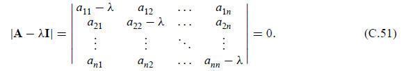
When this determinant is expanded, we obtain an algebraic polynomial equation in λ of degree n:

This is known as the characteristic equation of the matrix A. The left-hand side is called the characteristic
polynomial. We known that a polynomial of degree n has n (generally complex) roots λ₁, λ₂,
. . ., λ_n. These n numbers are called the eigenvalues, eigenroots or characteristic values of matrix A.
With each eigenvalue λ_i there is an associated vector x_i that satisfies

This x_i is called an eigenvector or characteristic vector. An eigenvector is unique only up to a scale
factor since if x_i is an eigenvector, so is βx_i where β is an arbitrary nonzero number. Eigenvectors are
often normalized so that their Euclidean length is 1, or their largest component is unity.

§C.4.1 Real Symmetric Matrices

Real symmetric matrices are of special importance in the finite element method. In linear algebra
books dealing with the algebraic eigenproblem it is shown that:
(a) The n eigenvalues of a real symmetric matrix of order n are real.
(b) The eigenvectors corresponding to distinct eigenvalues are orthogonal. The eigenvectors corresponding
to multiple roots may be orthogonalized with respect to each other.
(c) The n eigenvectors form a complete orthonormal basis for the Euclidean space E_n.

§C.4.2 Positivity

Let A be an n × n square symmetric matrix. A is said to be positive definite (p.d.) if

A positive definite matrix has rank n. This property can be checked by computing the n eigenvalues
λ_i of Az = λz. If all λ_i > 0, A is p.d.

A is said to be nonnegative if zero equality is allowed in (C.54):

A p.d. matrix is also nonnegative but the converse is not necessarily true. This property can be checked
by computing the n eigenvalues λ_i of Az = λz. If r eigenvalues λ_i > 0 and n−r eigenvalues are zero,
A is nonnegative with rank r .

A symmetric square matrix A that has at least one negative eigenvalue is called indefinite.

§C.4.3 Normal and Orthogonal Matrices

Let A be an n × n real square matrix. This matrix is called normal if

A normal matrix is called orthogonal if

All eigenvalues of an orthogonal matrix have modulus one, and the matrix has rank n.
The generalization of the orthogonality property to complex matrices, for which transposition is replaced
by conjugation, leads to unitary matrices. These are not required, however, for the material
covered in the text.

§C.5 THE SHERMAN-MORRISON AND RELATED FORMULAS

The Sherman-Morrison formula gives the inverse of a matrix modified by a rank-one matrix. The Woodbury
formula extends the Sherman-Morrison formula to a modification of arbitrary rank. In structural analysis these
formulas are of interest for problems of structural modifications, in which a finite-element (or, in general, a discrete
model) is changed by an amount expressable as a low-rank correction to the original model.

§C.5.1 The Sherman-Morrison Formula

Let A be a square n × n invertible matrix, whereas u and v are two n-vectors and β an arbitrary scalar. Assume
that Then

This is called the Sherman-Morrison formula when β = 1. Since any rank-one correction to A can be written as
, (C.58) gives the rank-one change to its inverse. The proof is by direct multiplication as in Exercise C.5.
For practical computation of the change one solves the linear systems Aa = u and Ab = v for a and b, using the
known . Compute . If , the change to A⁻¹ is the dyadic

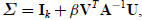
§C.5.2 TheWoodbury Formula

Let again A be a square n × n invertible matrix, whereas U and V are two n × k matrices with k ≤ n and β an
arbitrary scalar. Assume that the k ×k matrix in which denotes the k ×k identity matrix,
is invertible. Then

This is called the Woodbury formula. It reduces to (C.58) if k = 1, in which case Σ ≡ σ is a scalar. The proof
is by direct multiplication.

§C.5.3 Formulas for Modified Determinants

Let denote the adjoint of A. Taking the determinants from both sides of one obtains

If A is invertible, replacing this becomes

Similarly, one can show that if A is invertible, and U and V are n × k matrices,

Exercises for Appendix C: Determinants, Inverses, Eigenvalues

EXERCISE C.1
If A is a square matrix of order n and c a scalar, show that det(cA) = cⁿ detA.

EXERCISE C.2

Let u and v denote real n-vectors normalized to unit length, so that = u = 1 and = 1, and let I denote the
n × n identity matrix. Show that

EXERCISE C.3
Let u denote a real n-vector normalized to unit length, so that = u = 1 and I denote the n ×n identity matrix.
Show that

is orthogonal: H^TH = I, and idempotent: H² = H. This matrix is called a elementary Hermitian, a Householder
matrix, or a reflector. It is a fundamental ingredient of many linear algebra algorithms; for example the QR
algorithm for finding eigenvalues.

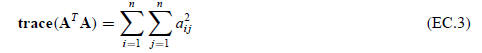
EXERCISE C.4
The trace of a n × n square matrix A, denoted trace(A) is the sum a_ii of its diagonal coefficients. Show
that if the entries of A are real,

EXERCISE C.5
Prove the Sherman-Morrison formula (C.59) by direct matrix multiplication

EXERCISE C.6
Prove the Sherman-Morrison formula (C.59) for β = 1 by considering the following block bordered system

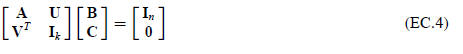
in which I_k and I_n denote the identy matrices of orders k and n, respectively. Solve (C.62) two ways: eliminating
first B and then C, and eliminating first C and then B. Equate the results for B.

EXERCISE C.7
Show that the eigenvalues of a real symmetric square matrix are real, and that the eigenvectors are real vectors.

EXERCISE C.8
Let the n real eigenvalues λ_i of a real n × n symmetric matrix A be classified into two subsets: r eigenvalues are
nonzero whereas n − r are zero. Show that A has rank r .

EXERCISE C.9
Show that if A is p.d., Ax = 0 implies that x = 0.

EXERCISE C.10
Show that for any real m × n matrix A, A^TA exists and is nonnegative.

EXERCISE C.11
Show that a triangular matrix is normal if and only if it is diagonal.

EXERCISE C.12
Let A be a real orthogonal matrix. Show that all of its eigenvalues λ_i , which are generally complex, have unit
modulus.

EXERCISE C.13
Let A and T be real n × n matrices, with T nonsingular. Show that T⁻¹AT and A have the same eigenvalues.
(This is called a similarity transformation in linear algebra).

EXERCISE C.14
(Tough) Let A be m × n and B be n × m. Show that the nonzero eigenvalues of AB are the same as those of BA
(Kahan).

EXERCISE C.15
Let A be real skew-symmetric, that is, A = −A^T . Show that all eigenvalues of A are purely imaginary or zero.

EXERCISE C.16
LetAbe real skew-symmetric, that is, Showthat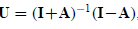called a Cayley transformation,
is orthogonal.

EXERCISE C.17
Let P be a real square matrix that satisfies

Such matrices are called idempotent, and also orthogonal projectors. Show that all eigenvalues of P are either
zero or one.

EXERCISE C.18
The necessary and sufficient condition for two square matrices to commute is that they have the same eigenvectors.

EXERCISE C.19
A matrix whose elements are equal on any line parallel to the main diagonal is called a Toeplitz matrix. (They
arise in finite difference or finite element discretizations of regular one-dimensional grids.) Show that if T₁ and
T₂ are any two Toeplitz matrices, they commute: T₁T₂ = T₂T₁. Hint: do a Fourier transform to show that the
eigenvectors of any Toeplitz matrix are of the form then apply the previous Exercise.